PostgreSQL Connections: Pooling and Saturation

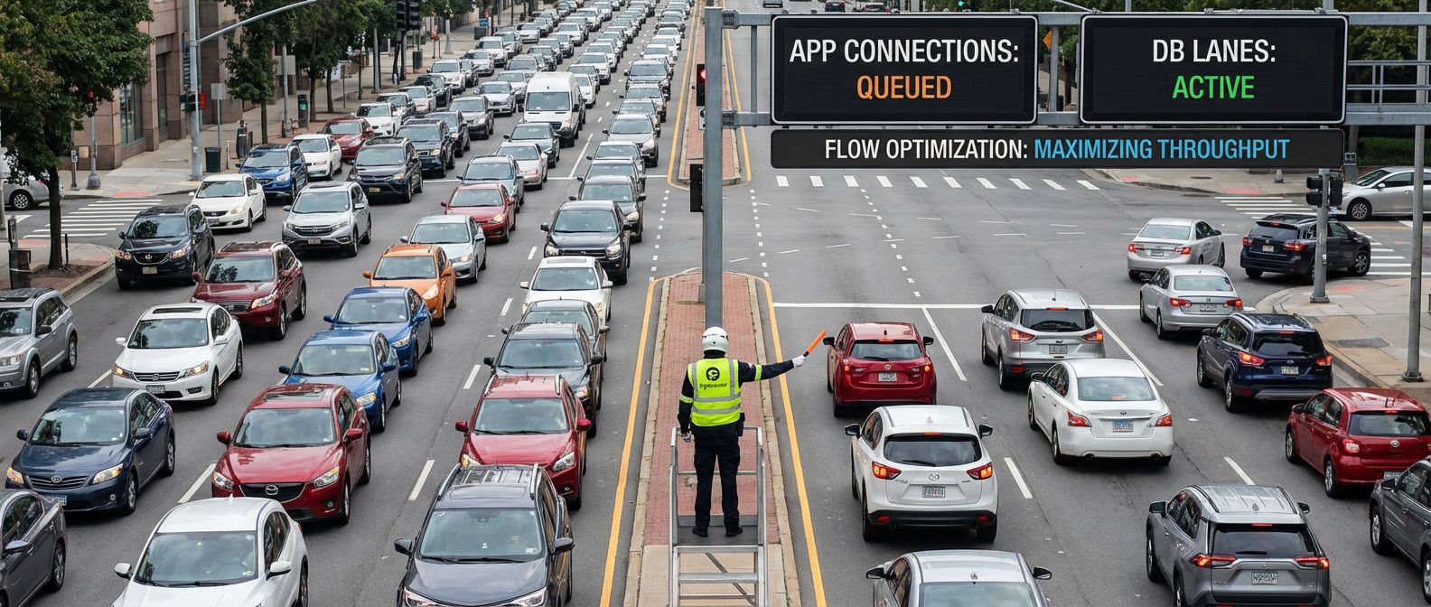
Table of Contents
Every PostgreSQL connection costs memory — roughly 5-10MB per connection — and requires a dedicated backend process. A database configured for 200 max connections isn’t “safe at 199.” It’s already under strain well before hitting that limit. Connection management isn’t about avoiding hard limits; it’s about understanding the soft degradation that happens as connections accumulate. Connection exhaustion doesn’t announce itself with a clean error. It manifests as slow queries, timeouts, and cascading failures across your application tier.
I’ve seen this pattern repeatedly: a team runs PostgreSQL with max_connections=200, comfortable at typical usage of 50. Traffic spikes, instances autoscale from 5 to 20, each with a pool of 20. Four hundred connections hit a 200 limit. Rejections cascade — threads block, health checks fail, more scaling triggers more connection requests.
The most common PostgreSQL scaling mistake: configuring max_connections high “just in case.” Each connection costs memory and CPU. A database with 1000 max_connections will perform worse than one with 200 — even at the same actual connection count — because of reservation overhead.
After adding PgBouncer, properly sizing pools, and implementing connection backpressure, the next traffic spike looks different. Database connections stay at 200. The application queues requests appropriately. Latency increases, but nothing fails.
Connection Fundamentals
How PostgreSQL Handles Connections
PostgreSQL uses a process-per-connection model. When a client connects, the main postgres process (the server daemon) forks a new backend process dedicated to that client. Each backend handles all queries for its connection (the TCP session between client and backend) until termination. In pg_stat_activity, these appear as rows with backend_type = 'client backend'. The fork-based model provides strong isolation — a crash in one backend doesn’t affect others — but it comes with overhead.
Establishing a new connection involves multiple steps: TCP handshake (1ms locally, 10-100ms over network), process fork (1-5ms), authentication (1-10ms depending on method), and TLS handshake if configured (5-50ms). Total: 10-200ms for a new connection. For web applications making dozens of queries per request, creating a fresh connection each time is prohibitively expensive.
Each backend process consumes resources independent of whether it’s actively running queries. The base memory footprint is roughly 5-10MB per connection, plus work_mem allocation when executing operations (4MB default, but can be much higher for complex queries). CPU overhead comes from OS scheduler contention — more backend processes means more context switching as the kernel cycles between them, even when most are idle.
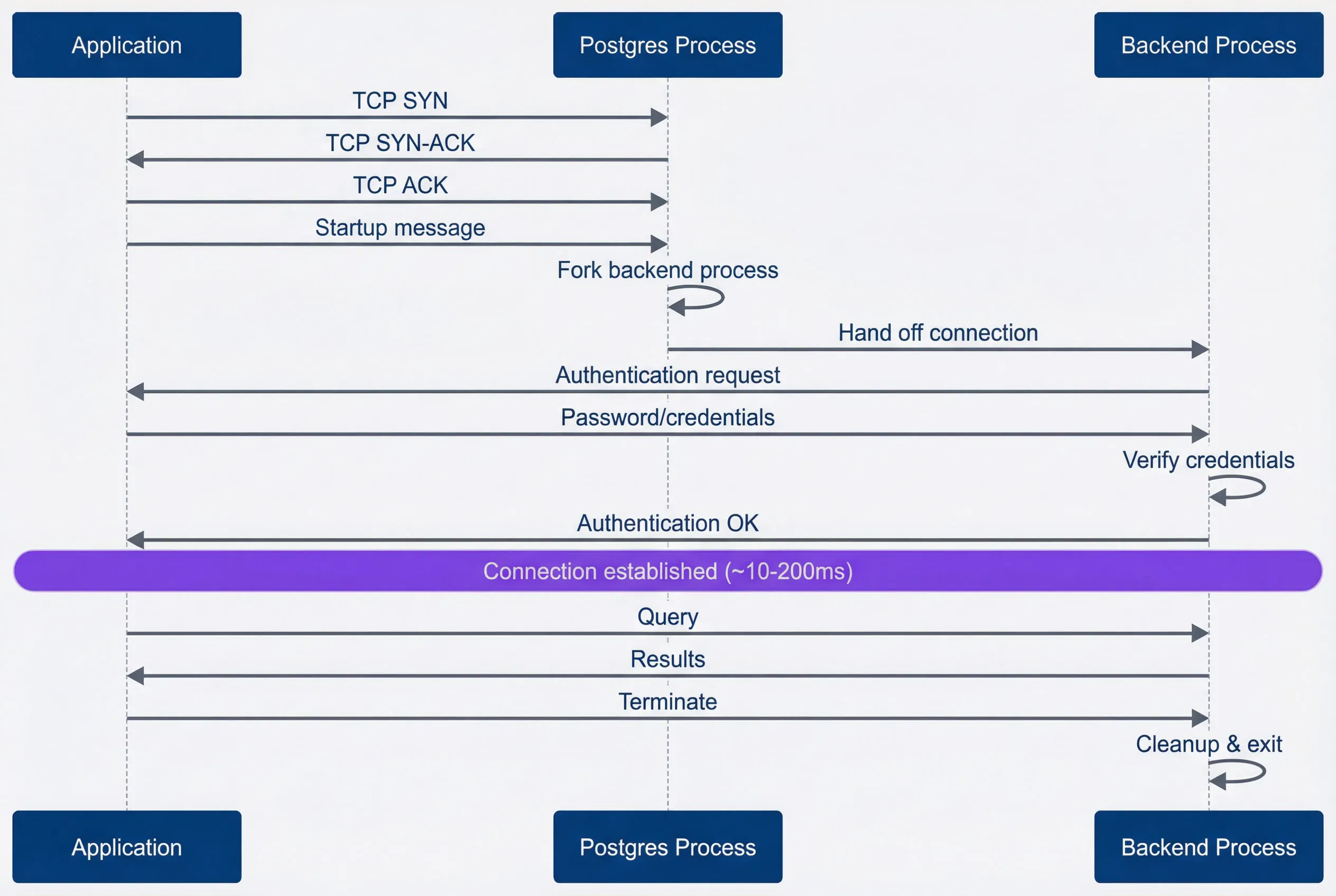
Connection establishment sequence.description
Sequence diagram with three participants: Application, Postgres Process, and Backend Process. The application starts a TCP handshake by sending TCP SYN to the Postgres process, which responds with TCP SYN-ACK, followed by the application sending TCP ACK. The application then sends a startup message to the Postgres process. The Postgres process forks a backend process and hands the connection off to that backend. The backend requests authentication from the application, the application sends password or credentials, the backend verifies those credentials, and then responds with Authentication OK. A note marks that the connection is now established in roughly 10 to 200 milliseconds. After establishment, the application sends a query to the backend and receives results. Finally, the application sends Terminate, and the backend performs cleanup and exits. The diagram shows the full overhead involved in creating a fresh PostgreSQL connection before useful query work begins.
The max_connections setting determines how many backend processes can exist simultaneously. The conventional wisdom is to set it high “for safety,” but this backfires. A database configured for 1000 connections reserves memory for 1000 potential backends even when only 50 are connected. The rule of thumb for bare metal: max_connections = (CPU cores × 2) + effective_spindle_count1. For SSDs, CPU cores × 4 works, but staying conservative (50-100) with a connection pooler is usually better.
| max_connections | Use Case | Memory Overhead | Notes |
|---|---|---|---|
| 50-100 | Small deployments with pooler | ~500MB-1GB | Recommended baseline |
| 100-300 | Medium deployments | ~1-3GB | Watch for contention |
| 500-1000 | Large deployments | ~5-10GB | Usually wrong; use pooler instead |
Connection Costs
Understanding where your connections come from — and what state they’re in — is critical for diagnosing saturation. The pg_stat_activity view shows all current connections with their state, user, application, and current query.
-- Current connection count by state
SELECT
    state,
    count(*) as connections,
    round(100.0 * count(*) / sum(count(*)) over(), 1) as percentage
FROM pg_stat_activity
WHERE backend_type = 'client backend'
GROUP BY state
ORDER BY connections DESC;

-- Connection count by application/user
SELECT
    usename,
    application_name,
    client_addr,
    count(*) as connections,
    count(*) FILTER (WHERE state = 'active') as active,
    count(*) FILTER (WHERE state = 'idle') as idle,
    count(*) FILTER (WHERE state = 'idle in transaction') as idle_in_txn
FROM pg_stat_activity
WHERE backend_type = 'client backend'
GROUP BY usename, application_name, client_addr
ORDER BY connections DESC;

-- Memory usage estimate (rough)
SELECT
    count(*) as total_connections,
    count(*) * 10 as estimated_memory_mb,
    current_setting('max_connections')::int as max_connections,
    round(100.0 * count(*) / current_setting('max_connections')::int, 1) as utilization_pct
FROM pg_stat_activity
WHERE backend_type = 'client backend';
Connection state tells you what each backend is doing. Most connections in a healthy pooled application should be idle—waiting for the next query. Active connections are executing queries; a high percentage of active connections indicates either long-running queries or genuine load.
| # | Connection State | Description | Concern Level |
|---|---|---|---|
| 1 | active | Executing query | Normal if short |
| 2 | idle | Waiting for query | Normal (pooled) |
| 3 | idle in transaction | Transaction open, no query | High (blocks vacuum) |
| 4 | idle in transaction (aborted) | Failed transaction, not rolled back | Critical |
“Idle in transaction” connections deserve special attention: they hold locks, prevent vacuum from cleaning up dead tuples, and consume connection slots. Set idle_in_transaction_session_timeout to kill them automatically.
Connection Pooling
Pooling Architectures
Connection pooling comes in two flavors: application-side pools and external poolers. Both solve the same problem — avoiding the overhead of creating new connections — but they scale differently.
- Application-side poolsLive within your application process. HikariCP (Java), node-postgres pool, SQLAlchemy (Python), and Go's database/sql all provide built-in pooling. The advantage is simplicity: no additional infrastructure, per-application configuration, and full support for prepared statements. The disadvantage is that scaling your application scales your connection count. Five application instances with pools of 20 connections each means 100 database connections. Twenty instances means 400. This couples your horizontal scaling to your database connection limits.
- External poolersSit between applications and the database as dedicated services. PgBouncer, Pgpool-II, and AWS RDS Proxy all work this way. The key benefit is connection multiplexing — many application connections can share fewer database connections. Your application can scale to 100 instances while the database sees a fixed 50 connections. The tradeoff is additional infrastructure and a potential single point of failure (mitigated by running multiple pooler instances).
- Managed database servicesOften provide built-in pooling. AWS RDS Proxy, Azure Database for PostgreSQL Flexible Server (with PgBouncer), and Google Cloud SQL don't offer native pooling but work well with Cloud SQL Auth Proxy for connection management. If you're on a managed platform, check whether pooling is available before deploying your own PgBouncer — the managed option is usually simpler to operate.
| Approach | Examples | Best For | Connection Scaling |
|---|---|---|---|
| Application-side | HikariCP, pg-pool, SQLAlchemy | Single app, prepared statements | instances × pool_size |
| External pooler | PgBouncer, RDS Proxy | Multi-app, auto-scaling | Fixed, independent of apps |
External poolers support different pooling modes that determine when connections are returned to the pool:
- Session modeClient gets a dedicated server connection for its entire session. No multiplexing benefit, but full prepared statement support. Use for long-running sessions or heavy prepared statement workloads.
- Transaction modeConnection returned after each transaction completes. High multiplexing, works for most web applications. Prepared statements work only with server-side preparation.
- Statement modeConnection returned after each statement. Maximum multiplexing but no multi-statement transactions. Use only for simple, stateless read workloads.
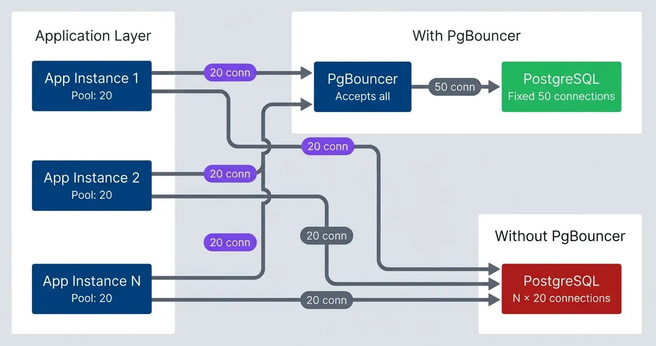
PgBouncer connection multiplexing.description
Top-to-bottom flowchart comparing direct PostgreSQL connections with pooled connections through PgBouncer. In the Application Layer group, App Instance 1, App Instance 2, and App Instance N each have a pool of 20 connections. In the Without PgBouncer group, each application instance connects directly to PostgreSQL, causing the database to accumulate N times 20 connections as application instances scale out. In the With PgBouncer group, the same application instances send their 20 connections each to PgBouncer, which accepts all incoming client connections and multiplexes them onto a fixed pool of 50 PostgreSQL connections. The direct PostgreSQL target is highlighted negatively, while the fixed 50-connection PostgreSQL target behind PgBouncer is highlighted positively. The diagram shows how PgBouncer decouples application scaling from raw database connection counts.
PgBouncer Configuration
PgBouncer configuration lives in pgbouncer.ini. The critical settings control connection limits, pooling behavior, and timeouts.
[databases]
myapp = host=postgres.internal port=5432 dbname=myapp

[pgbouncer]
; Connection limits
max_client_conn = 1000        ; Max client connections PgBouncer accepts
default_pool_size = 20        ; Server connections per pool (user+db combo)
min_pool_size = 5             ; Keep this many connections warm
reserve_pool_size = 5         ; Extra connections for burst handling
reserve_pool_timeout = 3      ; Seconds to wait before using reserve pool

; Pooling mode
pool_mode = transaction       ; session | transaction | statement

; Timeouts
server_idle_timeout = 600     ; Close idle server connections after 10 min
query_wait_timeout = 120      ; Max seconds client waits for connection
server_lifetime = 3600        ; Recycle connections after 1 hour

; Health checks
server_check_delay = 30
server_check_query = SELECT 1

; Admin interface
listen_addr = 0.0.0.0
listen_port = 6432
admin_users = pgbouncer_admin- Pool sizingFollows a simple formula: default_pool_size = PostgreSQL max_connections / number_of_pools. If PostgreSQL allows 100 connections and you have 5 user + database combinations (pools), each pool gets 20 connections. The reserve_pool handles burst traffic — set it to 10-25% of default_pool_size.
- max_client_connDetermines how many application connections PgBouncer accepts. This can be much higher than PostgreSQL's max_connections because PgBouncer queues requests when all server connections are busy. Set this based on peak concurrent application connections with headroom for spikes.
| Scenario | max_client_conn | default_pool_size | PostgreSQL max_connections |
|---|---|---|---|
| Small web app (5 instances) | 200 | 15 | 100 |
| Medium service (20 instances) | 500 | 25 | 200 |
| High scale (100+ instances) | 2000 | 50 | 400 |
Pool Sizing
Sizing Calculations
Pool sizing isn’t guesswork — it’s queuing theory. Little’s Law provides the foundation:
If your application handles 100 queries per second with an average query time of 50ms, you need
This is why the practical formula substitutes P99 query time for average: you want enough connections to handle 99% of queries without queueing, not just the typical case. Then double for variance and add burst capacity.
The practical formula for application pool sizing:
pool_size = ceil(peak_qps × p99_query_time × burst_factor)
For an application instance handling 50 queries per second at peak, with P99 query time of 100ms and a 2× burst factor: ceil(50 × 0.1 × 2) = 10 connections per instance.
| # | Factor | What to Measure | Impact |
|---|---|---|---|
| 1 | Query duration | P99 latency, not average | Longer queries need more connections |
| 2 | Request rate | Peak QPS, not average | Higher rate needs more connections |
| 3 | Variance | Standard deviation / mean | High variance needs more headroom |
| 4 | Burst factor | Peak / baseline ratio | Typically 2-3× for web traffic |
Common anti-patterns undermine even correct calculations:
- Oversized pools:Setting pool_size = 100 "just in case" means 10 instances create 1000 connections. Size based on actual need.
- No max lifetime:Connections held forever accumulate memory leaks and stale state. Recycle every 30 minutes.
- No idle timeout:Idle connections waste resources and hide leaks. Timeout after 10 minutes of inactivity.
Application Pool Configuration
Application-side pools need careful configuration. The pool library handles connection reuse, but you control the parameters that determine behavior under load.
import { Pool, PoolConfig } from 'pg'

const poolConfig: PoolConfig = {
  host: process.env.DB_HOST,
  port: parseInt(process.env.DB_PORT || '5432'),
  database: process.env.DB_NAME,
  user: process.env.DB_USER,
  password: process.env.DB_PASSWORD,

  // Pool sizing: peak_qps × p99_latency × burst_factor
  max: 20,
  min: 5,  // Keep pool warm

  // Timeouts
  connectionTimeoutMillis: 10000,  // Fail fast if pool exhausted
  idleTimeoutMillis: 30000,        // Reclaim idle connections
  // Note: pg-pool lacks maxLifetime; implement connection recycling
  // manually if needed (track connection age, close after 30min)

  // SSL for production
  ssl: process.env.NODE_ENV === 'production' ? {
    rejectUnauthorized: true,
    ca: process.env.DB_CA_CERT,
  } : false,
}

const pool = new Pool(poolConfig)

// Set statement timeout on new connections
pool.on('connect', (client) => {
  client.query('SET statement_timeout = 30000')
})

// Expose metrics for monitoring
function collectPoolMetrics() {
  return {
    total: pool.totalCount,
    idle: pool.idleCount,
    waiting: pool.waitingCount,
    utilization: pool.totalCount > 0
      ? (pool.totalCount - pool.idleCount) / pool.totalCount
      : 0,
  }
}

export { pool, collectPoolMetrics }For Java applications, HikariCP is the standard choice. It’s fast, well-maintained, and provides excellent metrics out of the box.
import com.zaxxer.hikari.HikariConfig;
import com.zaxxer.hikari.HikariDataSource;

public class DatabaseConfig {
    public static HikariDataSource createDataSource() {
        HikariConfig config = new HikariConfig();

        config.setJdbcUrl("jdbc:postgresql://localhost:5432/mydb");
        config.setUsername(System.getenv("DB_USER"));
        config.setPassword(System.getenv("DB_PASSWORD"));

        // Pool sizing
        config.setMaximumPoolSize(20);
        config.setMinimumIdle(10);

        // Timeouts
        config.setConnectionTimeout(10000);   // 10s to acquire connection
        config.setIdleTimeout(600000);        // 10min idle before removal
        config.setMaxLifetime(1800000);       // 30min max connection age

        // Validation
        config.setConnectionTestQuery("SELECT 1");
        config.setKeepaliveTime(300000);      // 5min keepalive

        // Leak detection
        config.setLeakDetectionThreshold(60000);  // Warn if held > 1min

        // Statement timeout
        config.addDataSourceProperty("options", "-c statement_timeout=30000");

        return new HikariDataSource(config);
    }
}Regardless of language or pool library, the same principles apply. These settings represent battle-tested defaults that work for most applications:
| Setting | Recommended Value | Rationale |
|---|---|---|
| max_pool_size | 10-30 per instance | Based on Little's Law calculation |
| min_pool_size | 50% of max | Keep pool warm, reduce latency |
| connection_timeout | 10s | Fail fast if pool exhausted |
| idle_timeout | 10-30 min | Reclaim unused connections |
| max_lifetime | 30 min | Prevent stale connections |
| leak_detection | 1-5 min | Catch unreturned connections |
Never set pool max_size to PostgreSQL max_connections. Leave headroom for admin connections, monitoring, migrations, and other applications. A good rule: application pools should use at most 80% of max_connections.
With pools configured, the next question is: how do you know if they’re working? Proper sizing is only half the battle — you need visibility into whether your pools have headroom or are approaching saturation.
Saturation Signals
Metrics to Monitor
Connection saturation doesn’t announce itself with a single metric. It’s a constellation of signals that, together, tell you whether your system has headroom or is approaching collapse. The goal is catching saturation early — before “too many connections” errors appear in logs.
- 1Connection utilizationThe primary signal. Query pg_stat_activity to compare current connections against max_connections. Alert at 70% utilization, investigate at 85%. By 95%, you're one slow query away from exhaustion.
SELECT
  count(*) AS current_connections,
  current_setting('max_connections')::int AS max_connections,
  round(100.0 * count(*) / current_setting('max_connections')::int, 1) AS utilization_pct
FROM pg_stat_activity
WHERE backend_type = 'client backend';- 2Pool wait timeMeasures how long requests wait for an available connection from the application pool. This metric comes from your pool library (HikariCP, pg-pool), not PostgreSQL. P99 wait time above 100ms indicates the pool is undersized; above 1 second means requests are timing out.
- 3Queue depthCounts requests waiting for connections. In PgBouncer, check cl_waiting. In application pools, check waitingCount or equivalent. Any sustained queue indicates saturation — the pool can't keep up with demand.
- 4Idle in transactionConnections are the silent killers. They hold connections hostage without doing work. Query for sessions stuck in this state for more than a minute — these are usually application bugs (missing commits, unclosed transactions in error paths).
SELECT pid, usename, application_name, state, query,
  now() - state_change AS idle_duration
FROM pg_stat_activity
WHERE state = 'idle in transaction'
  AND (now() - state_change) > interval '1 minute'
ORDER BY idle_duration DESC;Each metric has different thresholds for when to pay attention versus when to wake someone up at 3am. These thresholds are starting points — adjust based on your application’s tolerance for latency and your database’s capacity:
| # | Metric | Warning Threshold | Critical Threshold | Response |
|---|---|---|---|---|
| 1 | Connection utilization | > 70% | > 85% | Add pooler or reduce pool sizes |
| 2 | Pool wait time (P99) | > 100ms | > 1s | Increase pool size or optimize queries |
| 3 | Queue depth | > 10 | > 50 | Pool undersized or query bottleneck |
| 4 | Idle in transaction | > 5 connections | > 20 connections | Find and fix leaking transactions |
| 5 | Connection errors | Any occurrence | Sustained errors | Immediate investigation |
For PgBouncer deployments, the SHOW POOLS command exposes additional metrics. Watch cl_waiting (clients waiting for server connections), sv_idle (available server connections — zero means exhaustion), and maxwait (longest current wait time in seconds).
Monitoring Dashboard
During incidents, I need quick answers: Are connections the bottleneck? Are they being recycled? Is something blocking?
The connection snapshot query (see Reference Queries) gives a real-time breakdown of connection states and utilization — run this first during any database performance investigation.
Connection age distribution reveals recycling problems. If you see connections older than your max_lifetime setting (or hours/days old when you expect minutes), you have a leak or misconfiguration.
Lock blocking analysis identifies chains where one query holds locks that others are waiting for. When connections pile up, contention is often the culprit.
The progression from healthy to critical follows a predictable pattern:
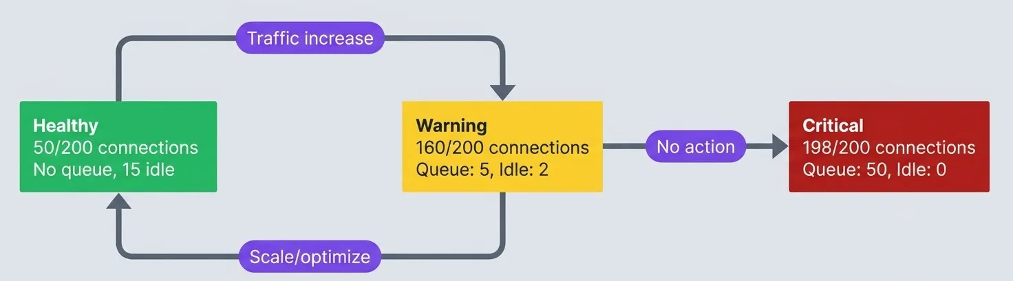
Connection saturation progression.description
Top-to-bottom flowchart showing three connection saturation states. The Healthy state shows 50 out of 200 connections in use, no queue, and 15 idle connections. A traffic increase moves the system from Healthy to Warning. The Warning state shows 160 out of 200 connections in use, a queue of 5, and 2 idle connections. From Warning, if no action is taken, the system progresses to Critical. The Critical state shows 198 out of 200 connections in use, a queue of 50, and 0 idle connections. There is also a recovery path from Warning back to Healthy labeled Scale or optimize. The healthy state is highlighted positively, the warning state is highlighted as cautionary, and the critical state is highlighted negatively. The diagram explains how connection exhaustion develops gradually and where intervention can restore normal operation before the database reaches saturation.
Failure Patterns
Connection Exhaustion Cascade
Connection exhaustion rarely happens in isolation. It cascades. Understanding the stages helps you recognize where you are in the failure progression and what interventions are still possible.
- Stage 1: SaturationBegins with a traffic spike or slow queries. Pool utilization climbs. Connection wait times increase. Query latencies creep up. This stage can last minutes to hours, giving you time to respond if you're watching the right metrics.
- Stage 2: QueueingStarts when the pool is fully utilized. Requests begin queuing for connections. Request latencies spike. Timeout errors appear sporadically. This stage lasts seconds to minutes — your window for intervention is shrinking.
- Stage 3: TimeoutsHit when the queue exceeds timeout thresholds. Connection timeout errors multiply. Transactions abort mid-flight. Users see errors. The system is now visibly failing.
- Stage 4: CascadeWhere things get worse before they get better. Applications retry failed requests, compounding the problem. Retry storms create more connection demand. Health checks fail. Kubernetes kills and restarts pods, which then all try to establish connections simultaneously. The problem feeds itself.
- Stage 5: CollapseMeans complete unavailability. The database refuses all new connections. Recovery requires manual intervention:
Once you reach Stage 5, the instinct is to restart everything at once. Resist it. A “thundering herd” recovery — where every application instance reconnects simultaneously — recreates the exact conditions that caused the collapse. Each instance tries to fill its connection pool, slamming the database with hundreds of concurrent connection requests before it has finished cleaning up the previous mess. The recovery playbook matters as much as the prevention strategy, and it follows a specific sequence:
- 1Stop the bleedingScale application instances to zero or block traffic at the load balancer. This stops new connection attempts.
- 2Clear stuck connectionsOn PostgreSQL, run SELECT pg_terminate_backend(pid) FROM pg_stat_activity WHERE state = 'idle in transaction' AND state_change < now() - interval '5 minutes'; to kill stuck sessions.
- 3Restart applications graduallyBring up one instance, verify it connects and serves traffic, then add more. Don't start all instances simultaneously — they'll all try to fill their pools at once.
- 4Monitor during recoveryWatch pg_stat_activity connection count as you add instances. Stop scaling if you approach 80% utilization.
Recovery gets you back to operational, but it doesn’t prevent the next incident. The cascade pattern repeats because the underlying architecture lacks defensive layers — there’s nothing between “working fine” and “total collapse.” Building resilience means adding checkpoints where the system can absorb pressure instead of transmitting it. Each layer below addresses a different failure mode, and they compound: connection limits cap the blast radius, circuit breakers stop the bleeding, backpressure prevents the bleeding from starting, and graceful degradation keeps users served even when the database is under strain.
- Connection limitsSet maximums at application pools, PgBouncer, and PostgreSQL. The principle is "fail fast at the application, not the database."
- Circuit breakersDetect saturation and return fast errors instead of queueing. Let the system recover.
- BackpressureRate limit at the ingress. Use bounded queues. Shed load during saturation.
- Graceful degradationDisable non-critical features under stress. Serve cached responses. Return partial results.
Recovery Strategies
When saturation hits, you need patterns that prevent cascade failures. These aren’t theoretical — they’re the difference between a slow day and a multi-hour outage.
Circuit breakers stop the bleeding. When connection errors exceed a threshold, the circuit “opens” and immediately rejects requests instead of queuing them. This gives the database breathing room to recover. After a timeout, the circuit enters a “half-open” state, allowing a few requests through to test whether the database has recovered.
Circuit breakers for database connections live in your application code, wrapping the connection pool. They’re not implemented in PgBouncer (which has no circuit breaker concept) or at the ingress controller (which operates at HTTP level, not database protocol). The application is the right place because it understands the difference between a transient connection timeout and a sustained outage.
The essential logic: track consecutive failures, “open” the circuit after a threshold, reject requests immediately while open, then periodically test with a single request to see if the database has recovered.
// Circuit breaker wraps the pool, not individual queries
const breaker = new DatabaseCircuitBreaker({ threshold: 5, timeout: 30000 })
const pool = new Pool(poolConfig)

// All database access goes through the breaker
async function getUser(id: string) {
  return breaker.query(pool, 'SELECT * FROM users WHERE id = $1', [id])
}Retry budgets prevent retry storms. Instead of retrying every failed request, track the ratio of retries to total requests. When retries exceed 20% of traffic, stop retrying — you’re making things worse. Wire the retry budget into your circuit breaker:
const budget = new RetryBudget({ windowMs: 60000, maxRetryRatio: 0.2 })

async function queryWithRetry<T>(sql: string, params?: unknown[]): Promise<T> {
  budget.recordRequest()
  try {
    return await breaker.query<T>(pool, sql, params)
  } catch (error) {
    if (budget.canRetry() && isRetryable(error)) {
      budget.recordRetry()
      return breaker.query<T>(pool, sql, params)  // Single retry attempt
    }
    throw error
  }
}Each failure scenario has a different detection method and response. The key is matching the response to the root cause:
| Scenario | Detection | Response | Recovery |
|---|---|---|---|
| Slow queries | Wait time > threshold | Add query timeout | Optimize queries |
| Connection leak | Idle-in-txn > limit | Kill sessions | Fix application code |
| Traffic spike | Utilization > 80% | Shed load | Scale or add pooler |
| Database overload | Connection errors | Circuit break | Scale database |
Conclusion
PostgreSQL connection management is a critical but often neglected aspect of application architecture. Most teams don’t think about it until 3am when the database stops accepting connections.
The key insights from this article:
- Connections are expensive.—
Each connection costs 5-10MB of memory, consumes CPU through context switching, and competes for shared resources. The counterintuitive truth: fewer connections often means better performance. Keep
max_connectionslow and use pooling. - Pooling decouples application scaling from database limits.—
PgBouncer (or similar external poolers) lets you scale application instances without proportionally increasing database connections. Transaction pooling mode handles most workloads well.
- Size pools with math, not intuition.—
Little’s Law (
) gives you a starting point. Account for variance with a burst factor. Anti-patterns like oversized pools (“just in case”) create more problems than they solve. - Monitor saturation, not just errors.—
By the time you see “too many connections” errors, you’re already in a cascade. Set alerts on the utilization thresholds discussed earlier. Watch for idle-in-transaction sessions — they’re connection leaks waiting to bite you.
- Design for graceful degradation.—
Circuit breakers, retry budgets, and backpressure turn connection exhaustion from a hard failure into a soft degradation. Build these patterns before you need them.
The goal isn’t to handle unlimited connections — it’s to handle connection constraints gracefully, so saturation causes slowdowns, not outages.
Connection management is about building slack into the system. A database running at 90% connection capacity has no room for variance, spikes, or slow queries. Target 50-70% utilization to leave room for reality to differ from expectations.
Reference Queries
These SQL queries are useful for monitoring and debugging PostgreSQL connection issues. Run them against your database during incidents or as part of regular health checks.
Connection Snapshot
Real-time breakdown of connection states and utilization:
SELECT
  count(*) AS total_connections,
  count(*) FILTER (WHERE state = 'active') AS active,
  count(*) FILTER (WHERE state = 'idle') AS idle,
  count(*) FILTER (WHERE state = 'idle in transaction') AS idle_in_txn,
  current_setting('max_connections')::int AS max_conn,
  round(100.0 * count(*) / current_setting('max_connections')::int, 1) AS utilization_pct
FROM pg_stat_activity
WHERE backend_type = 'client backend';
Connection Age Distribution
Identifies connections that aren’t being recycled:
SELECT
  CASE
    WHEN age < interval '1 minute' THEN '< 1 min'
    WHEN age < interval '10 minutes' THEN '1-10 min'
    WHEN age < interval '1 hour' THEN '10-60 min'
    WHEN age < interval '1 day' THEN '1-24 hours'
    ELSE '> 1 day'
  END AS age_bucket,
  count(*) AS connections
FROM (
  SELECT now() - backend_start AS age
  FROM pg_stat_activity
  WHERE backend_type = 'client backend'
) ages
GROUP BY 1
ORDER BY min(age);Lock Blocking Analysis
Finds queries blocking other queries:
WITH blocked AS (
  SELECT
    blocked.pid AS blocked_pid,
    blocked.query AS blocked_query,
    blocking.pid AS blocking_pid,
    blocking.query AS blocking_query,
    now() - blocked.state_change AS blocked_duration
  FROM pg_stat_activity blocked
  JOIN pg_locks blocked_locks ON blocked.pid = blocked_locks.pid
  JOIN pg_locks blocking_locks
    ON blocked_locks.locktype = blocking_locks.locktype
    AND blocked_locks.database IS NOT DISTINCT FROM blocking_locks.database
    AND blocked_locks.relation IS NOT DISTINCT FROM blocking_locks.relation
    AND blocked_locks.pid != blocking_locks.pid
  JOIN pg_stat_activity blocking ON blocking_locks.pid = blocking.pid
  WHERE NOT blocked_locks.granted
)
SELECT * FROM blocked
WHERE blocked_duration > interval '10 seconds'
ORDER BY blocked_duration DESC;Kill Stuck Sessions
Emergency cleanup of idle-in-transaction sessions (use with caution):
SELECT pg_terminate_backend(pid)
FROM pg_stat_activity
WHERE state = 'idle in transaction'
AND state_change < now() - interval '5 minutes';Footnotes
-
Effective spindle count represents the hardware’s capacity for concurrent I/O requests. A traditional HDD has one spindle and can usually only handle one I/O request at a time. For modern SSD-based storage, this metric is often considered 0 or ignored in the original formula. Because SSDs handle many parallel I/O requests, some modern benchmarks suggest using I/O queue depth as a more relevant replacement.
↩
Sharethisarticle
Enjoyed the read? Share it with your network.